-
PDF
- Split View
-
Views
-
Cite
Cite
Stan Kotwicki, James N. Ianelli, André E. Punt, Correcting density-dependent effects in abundance estimates from bottom-trawl surveys, ICES Journal of Marine Science, Volume 71, Issue 5, July/August 2014, Pages 1107–1116, https://doi.org/10.1093/icesjms/fst208
Close - Share Icon Share
Abstract
Indices of abundance are important for estimating population trends in stock assessment and ideally should be based on fishery-independent surveys to avoid problems associated with the hyperstability of the commercial catch per unit effort (cpue) data. However, recent studies indicate that the efficiency of the survey bottom trawl (BT) for some species can be density-dependent, which could affect the reliability of survey-derived indices of abundance. A function qe∼f(u), where qe is the BT efficiency and u the catch rate, was derived using experimentally derived acoustic dead-zone correction and BT efficiency parameters obtained from combining a subset of BT catch data with synchronously collected acoustic data from walleye pollock (Theragra chalcogramma) in the eastern Bering Sea (EBS). We found that qe decreased with increasing BT catches resulting in hyperstability of the index of abundance derived from BT survey. Density-dependent qe resulted in spatially and temporarily variable bias in survey cpue and biased population age structure derived from survey data. We used the relationship qe∼f(u) to correct the EBS trawl survey index of abundance for density-dependence. We also obtained a variance–covariance matrix for a new index that accounted for sampling variability and the uncertainty associated with the qe. We found that incorporating estimates of the new index of abundance changed outputs from the walleye pollock stock assessment model. Although changes were minor, we advocate incorporating estimates of density-dependent qe into the walleye pollock stock assessment as a precautionary measure that should be undertaken to avoid negative consequences of the density-dependent qe.
Introduction
Indices of abundance are important for estimating population trends in stock assessment and hence fishery management. Ideally, abundance indices should be based on fishery-independent data collection methods such as design-based surveys (Maunder and Punt, 2004). Indices based on commercial fishery catch per unit effort (cpue) should be avoided, since they are unlikely to be proportional to actual abundance (Beverton and Holt, 1957; Peterman and Steer, 1981; Swain and Sinclair, 1994; Harley et al., 2001; Maunder and Punt, 2004) and may fail to reflect changes in abundance due to “hyperstability” or “hyperdepletion” (Hilborn and Walters, 1992). Hyperstability represents situation when cpue stays high as abundance drops, whereas for hyperdepletion, cpue drops much faster than abundance. Stock assessments relying on such data may fail to track population changes and could lead to fishery collapse or underutilization (Hutchings, 1996; Walters and Maguire, 1996; Erisman et al., 2011). Fishery-independent bottom-trawl (BT) surveys, which are assumed to be proportional to abundance, have been widely used to provide indices of abundance to avoid problems associated with the hyperstability or hyperdepletion of the commercial cpue data (Godø, 1994; Ianelli et al., 2012). However, density-dependent effects in survey BT operations may also result in hyperstable indices of abundance (Kotwicki et al., 2013) similar to those observed with commercial cpue data.
Density-dependent effects of the BT have been identified as factors that may affect the reliability of abundance estimates from BT surveys (Godø et al., 1990; Godø and Wespestad, 1993; Godø, 1994; Aglen et al., 1997; Kotwicki et al., 2013). For example, survey trawl capture efficiency for Atlantic cod (Gadus morhua) and haddock (Melanogrammus aeglefinus) increases with fish density (Godø et al., 1999). The opposite effect was observed for capelin (Mallotus villosus; O'Driscoll et al., 2002), Atlantic croakers (Micropogonias undulatus), white perch (Morone americana; Hoffman et al., 2009), and walleye pollock (Theragra chalcogramma; Kotwicki et al., 2013). Despite these findings, evaluations of the spatial and temporal variability in density-dependent BT survey efficiency are lacking, and methods which correct time-series of survey abundance indices are unavailable.
The derivation of a relative index of abundance from a fishery-independent survey is based on the relationship u = qD, where u is the catch rate (fish density) detected by the BT, D the true density, and q a proportionality constant, usually referred to as catchability (Punt and Hilborn, 1997). Catchability is often decomposed into two components q=qaqe, (Godø, 1994), where qa is the availability to the BT [i.e. the proportion of fish in the water column present between the bottom and effective fishing height (EFH) of the BT; hereafter, it is referred to as BT zone (BTZ)] and qe the BT efficiency (the proportion of fish in the BTZ caught by the trawl). Catchability is unknown for most fishery-independent surveys, but it is often assumed to be stationary in time and space (Kimura and Somerton, 2006). This assumption can be critical for stock assessments, spatial dynamics studies, and ecological modelling (Kotwicki et al., 2013). Estimates of abundance trends may be misleading if either qe or qa of the BT is affected by density (Godø, 1994). Consequently, methods for estimating qe and correcting survey-derived indices of abundance for density-dependence are needed.
Developing an estimator for qe is difficult because this requires independent measures of fish density in the BTZ (Somerton et al., 1999). Past studies estimating qe for semi-pelagic species have used independent estimates of abundance in front of the BT derived from acoustic backscatter data within the BTZ (O'Driscoll et al., 2002; Hoffman et al., 2009; Doray et al., 2010). To avoid biases, these data need to be relatively free from contamination by other species and need to have an estimate of the acoustic dead-zone correction (Ona and Mitson, 1996; Kotwicki et al., 2013). The methods are difficult to apply because most time-series of the BT survey data lack acoustic measurements. In addition, backscatter data from many survey tows are often contaminated by other organisms even if acoustic data are available. Consequently, BT efficiency is usually estimated in an experimental manner outside of standard survey operations (O'Driscoll et al., 2002) or alternatively for a subset of tows where contamination (in the backscatter) from other species can be assumed negligible (Hoffman et al., 2009). If estimates of qe were provided for all tows within the survey time-series, a more reliable index of abundance could be available for stock assessments and ultimately fishery management.
The purpose of this investigation is to produce a more reliable BT survey index for walleye pollock (hereafter referred to as “pollock”) in the eastern Bering Sea (EBS) by extending on Hoffman et al. (2009) and O'Driscoll et al. (2002) to incorporate experimentally derived acoustic dead-zone corrections and BT efficiency parameters derived from combining acoustic and BT survey data (Kotwicki et al., 2013). Our method incorporates uncertainty associated with the estimation of the acoustic dead-zone correction and BT efficiency parameters. We also obtain estimates of qe for all tows in the survey time-series by modelling the relationship between survey cpue and qe. We postulate that qe,i = f(ui), where i indicates a survey tow when qe is density-dependent. From this relationship, we estimate qe,i for all tows in a survey time-series and hence new estimates of total BT survey abundance. The secondary goal of this paper is to assess if density-dependent qe for pollock in the EBS leads to a hyperstable index of abundance by assessing the relationship between mean survey catching efficiency and corrected index of abundance. Pollock was chosen for this investigation because it is a key species in Subarctic Pacific ecosystems and supports a substantial fishery that accounts for ∼5% of global fish harvest, with annual harvests ranging from 4 to 7 million tonnes (Bailey et al., 1999). It ranked second in the world among marine species in capture production in 2008 (FAO, 2010).
Methods
Data
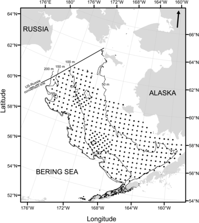
The EBS BT survey has been conducted annually over a standard grid of stations since 1982 (Lauth and Nichol, 2013). Most of the 376 survey stations were located at the centres of a 20 × 20 nautical mile grid (Figure 1). Stations at the corners of the grids were also sampled in two regions (near St Matthew Island and the Pribilof Islands). The surveys are conducted annually in June and July using a standardized sampling gear (the 83–112 Eastern otter trawl). The survey stations are visited beginning with those in the northeastern corner (Bristol Bay) of the area then proceeding westward. The standard tow duration is 30 min on bottom, and the tow speed is 1.54 m s–1 (3 knots; see Lauth and Nichol, 2013, for details). During 2005–2009, acoustic backscatter data were collected annually for all BT hauls. A detailed description of acoustic data processing is given in Kotwicki et al. (2013).
Abundance indices
Total population estimates from the EBS BT survey (hereafter referred to as the status quo index of abundance) were derived using methods detailed in Wakabayashi et al. (1985). In brief, the catch rates are calculated as ui = ni/Ei, where ni is the number of pollock caught in tow i and Ei the corresponding fishing effort. Haul effort was based on area-swept estimates (Godø and Engås, 1989), defined as the product of tow distance and average net width measured with acoustic sensors (Kotwicki et al., 2011). Mean stratum catch rates (in no. hectare–1) weighted by the stratum area were combined to estimate the total abundance. Variances and coefficients of variation (CVs) around abundance estimates were calculated assuming stratified random sampling to assure consistency with the currently used methods for variance estimation in pollock EBS surveys (for details, see Wakabayashi et al. 1985).
Population-at-age estimates were derived using methods described by Wakabayashi et al. (1985) and Kimura (1989). In brief, length frequencies were weighted by cpue for each tow and combined across tows to estimate population at length. Yearly age–length keys (combined over entire survey area) were then applied to compute numbers by age and length class by strata. Finally, these data were summed over strata to estimate total survey area population at age.
Estimating BT efficiency using acoustic data
New abundance estimates
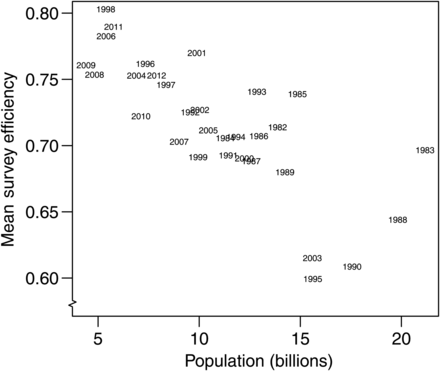
Since mean abundance replicates represent a corrected distribution of the survey process, the mean and variance provide an alternative index of abundance (hereafter referred to as the new index of abundance) to use within the stock assessment model (Ianelli et al., 2012). To determine if the status quo index was hyperstable, the new index was contrasted with the status quo BT survey index. The hyperstable index detects changes in the population abundance that are smaller than actual changes in the population abundance (Hilborn and Walters, 1992). To determine if the status quo index was hyperstable, mean BT survey catching efficiency (i.e. the ratio of the status quo index over the new index) was plotted against the status quo index because the negative slope of this relationship would indicate the hyperstability of the status quo index.
Estimation of the population age structure of a new index of abundance
We explored the impact of the variability in qe among tows and the tendency of pollock to form dense schools by age class on the estimated survey proportions-at-age by year. This was done by sampling |${\dot u_i}$| vectors, and applying the methodology described above to estimate mean qe by age for each survey year and the means of the distributions of the proportions-at-age.
Effect of the new BT index on stock assessment model output
The effect of replacing the status quo BT index of abundance with the new BT index in the stock assessment was investigated for the three BT survey data inputs: abundance, age structure, and the variance–covariance matrix. The assessment was run three times, replacing model inputs to explore the impact of each component. In the first run, we replaced only the total abundance estimates; in the second run, we replaced total abundance estimates and age structure; and in the third, we replaced all three inputs. The outputs from the runs of the assessment were compared in terms of the estimates of spawning-stock biomass (SSB) and the CVs of three estimates.
Results
BT efficiency
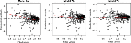
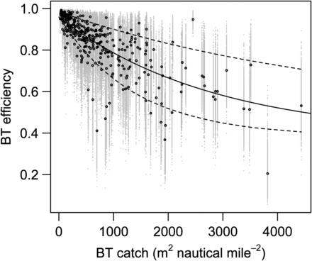
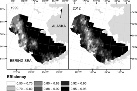
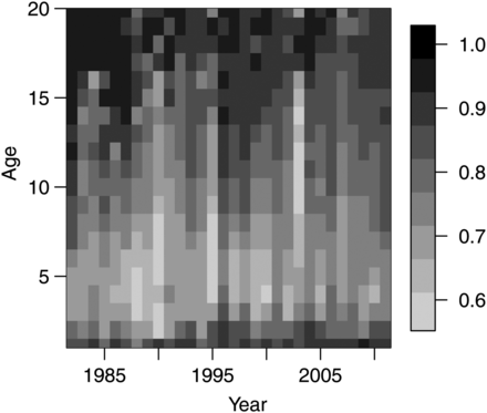
Likelihood ratio tests (p-value = 0.0031) and a lack of a trend in the residuals (Figure 2) indicated that the three-parameter model (7c) was the best of the models considered [see Table 1 for mean parameter β values and their s.d. for model (7c)]. The qe, which is close to 1 for very low catches decreases exponentially with catch (Figure 3) and asymptotically approaches 0.44 at extremely large catches. The parameter qe varied spatially within the range of 0.50–0.98 (Figure 4) and temporally within similar range (results not shown). Examples presented on Figure 4 show that qe in 1999 and 2012 varied spatially; however, spatial distribution of qe was different between years, indicating temporal variability in qe across years. Furthermore, qe varied with pollock age and was generally lowest for ages between 3 and 8, with large interannual variability (Figure 5).
Posterior mean parameter values and posterior standard deviations for parameters in model (7c).
| Parameter . | β0 . | β1 . | β2 . |
|---|---|---|---|
| Mean | 0.447 | 0.00046 | 0.645 |
| Standard deviation | 0.035 | 0.00014 | 0.059 |
| Parameter . | β0 . | β1 . | β2 . |
|---|---|---|---|
| Mean | 0.447 | 0.00046 | 0.645 |
| Standard deviation | 0.035 | 0.00014 | 0.059 |
Standardized residuals against fitted values for models (7a), (7b), and (7c).
MCMC-derived vectors of BT efficiency vs. BT catch. Black and grey points, respectively, represent the mean and all estimates of BT efficiency (qe) from the MCMC samples. The black line represents the fit of model (7c) to the means, and dashed lines represent 95% confidence bounds around model predictions of qe.
Examples of distribution of EBS survey BT efficiency (qe) from years 1999 and 2012.
New abundance estimates
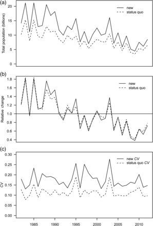
The new index of total abundance was consistently larger in absolute terms than the status quo index (Figure 6a), but the trends in relative abundance were very similar (Figure 6b). With the respect to the mean, the new index tended to be higher than the status quo index when the latter was high and lower when it was low, indicating evidence of hyperstability in the status quo index (Figure 6b). The hyperstability was confirmed by a negative trend in the relationship between mean survey efficiency and population abundance (Figure 7). Year-specific CVs for the status quo index and from the diagonal of the ∑u matrix indicated that the uncertainty around the new index increased by 55% on average (Figure 6c). This increase was highly variable and ranged from 30% in 2009 to 102% in 1997.
(a) Time-series of new vs. status quo total abundance estimates, (b) change relative to the mean abundance across the time-series, and (c) new vs. status quoCV.
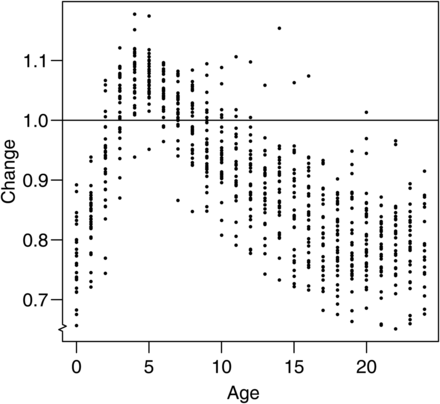
The population age structure, represented by proportions-at-age, differed markedly between the status quo and new series (Figure 8). Abundance at age for ages 3–8 for the new index was generally larger, whereas the abundance at age for the other ages was generally smaller.
Relative change in the proportion of abundance at age (new divided by status quo) for EBS survey time-series. Each dot represents a survey year. Horizontal line represents no change.
Effect of the new index on stock assessment model output
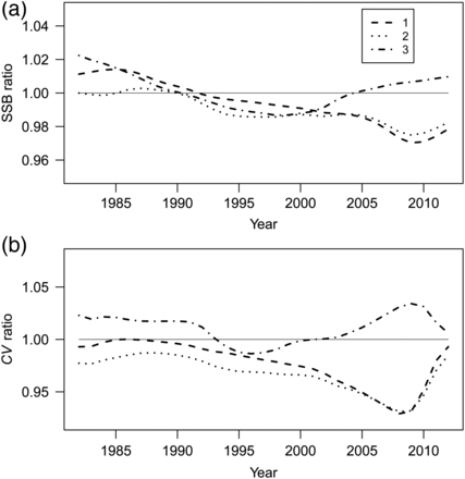
As expected, the replacement of the status quo index with the new index of abundance indicates that the BT index is hyperstable. However, the consequences of the extent of hyperstability appear to be small in the pollock stock assessment because the differences in SSB estimates were less than 3% (Figure 9a). The replacement of the status quo abundance estimates with the new index resulted in increased SSB estimates during the early part of the time-series (when abundance was highest) and decreased estimates of SSB for the years after 1990 (Figure 9a; line 1). The addition of the new proportions-at-age had little effect on the SSB (Figure 9a; line 2). Finally, the replacement of all three new components of the index (abundance, age structure, and variance–covariance matrix) resulted in changes similar to those observed in line 1 up to year 2004, but estimates of SSB after 2004 were higher. The CV for SSB decreased for almost all years when the abundance and proportion-at-age time-series were replaced (Figure 9b; lines 1 and 2). However, the inclusion of a variance–covariance matrix led to higher CVs for both the early and most recent years and lower CVs between 1992 and 2000 (Figure 9b; line 3).
Ratio of SSB (upper panel) and CV of SSB (lower panel) estimated from the the stock assessment using the new index of abundance relative to that estimated from status quo. Line 1 represents a ratio when only abundance estimates were replaced. Line 2 represents a ratio when abundance estimates and age structure were replaced. Line 3 represents a ratio when abundance estimates, age structure, and variance structure were replaced.
Discussion
Density-dependence of the BT survey catchability is a potential source of concern because it causes a systematic bias in BT cpue that could lead to bias in the assessment results and subsequent management advice. This bias increases with increasing fish density for pollock in the EBS resulting in a non-linear negative relationship between qe and fish density. This relationship violates a major assumption that BT survey cpue is proportional to fish density and that q does not change in space or in time (Wilberg et al., 2010). The consequences of this could be serious for a wide range of products derived from BT survey data because the effect of variable qe impacts cpue estimates at an individual station level. These include, but are not limited to, stock assessments that use abundance estimates at age and their variances (Godø et al., 1999; Ianelli et al., 2012), studies of density-dependent effects on distribution (Spencer, 2008; Kotwicki and Lauth, 2013), density-dependent mortality (Myers and Cadigan, 1993), recruitment (Myers, 2001), and ecological studies on density-dependent interactions between species (Ressler et al., 2012). Below, we will review some major implications of our findings for two types of users: those who use the BT survey data as an index of abundance over the entire survey area and those who use spatially explicit cpue data as a measure of fish density at particular sampling locations.
Survey-wide index of abundance
Survey-wide indices of abundance are used for management purposes in stock assessments. Our results indicate that density-dependence in qe can impact stock assessments in three ways by (i) causing an index of abundance to become hyperstable, (ii) providing biased estimates of the age structure of the population, and (iii) causing (spatial and) temporal variability in survey catchability. Fishery-independent surveys have been thought not to be hyperstable (Harley et al., 2001). However, our findings suggest that this assumption may not always be valid. Relative to the mean, changes in abundance between years detected by the new index were larger than those detected by the status quo index (Figure 6b), indicating hyperstability (Hilborn and Walters, 1992). Besides problems with detecting the correct magnitude of the change in abundance from year to year, a hyperstable BT survey-based index of abundance could also infer false trends. For example, a hyperstable index would increase if mean fish densities were the same between 2 years, but fish were more aggregated in the first year and more dispersed in the second because mean trawl efficiency would be higher during the more dispersed year. The changes in the SSB estimates that we observed in the pollock assessment suggest that the status quo BT index is hyperstable, although the magnitude of the effect seems to be relatively minor (<3%). Nevertheless, ignoring density-dependence of the survey BT qe would be imprudent. Abundance indices corrected for density-dependence in the presence of a negative correlation between qe and fish density provide a better chance for detecting changes in stock size and hence provide better advice for management.
High variability in the mean BT survey efficiency evident in Figure 7 indicates that density-dependence in qe may lead to situations other than hyperstability. For example, the population estimate for 1983 was twice that for 1999, but mean survey efficiency for both years was similar. This was possible because of temporal variability in qe (Figure 4). Moreover, temporal variability in survey qe can lead to detection of false trends in population size among years. For example, corrected population estimates for 1985 and 1995 were approximately equal at 15 billion fish, but the uncorrected estimates were 11.2 and 9.5 billion fish, respectively. This temporal variability in qe implies additional uncertainty about the index of abundance that is unaccounted for by sampling variability. Therefore, the estimates of uncertainty should include two sources: that from sampling variability and that from uncertainty associated with the estimate of survey efficiency. The increase in the CV of the new index ranged between 30 and 102%. This indicates that ignoring the contribution of uncertainty in qe may also lead to bias in the stock assessment models, particularly the estimates of uncertainty. The need to account for the other sources of variability in the assessment models has been shown previously by Punt et al. (2005), where they attribute this additional variation to fluctuations in catchability and estimate it as an additional parameter in the assessment. Here, we accounted for what is likely to be the two main sources of variation, but acknowledge that other sources may exist. For example, uncertainty may also arise from the second component of q: qa. For semi-pelagic species such as pollock, qa depends on variability in the proportion of fish from the entire water column that are present in the BTZ, which depends on factors such as light level and fish length (Kotwicki et al., 2009). Lastly, the fact that different proportions of the resource may be present from year to year in the area surveyed can also result in an overly-optimistic impression of the precision of the survey index of abundance (Geromont and Butterworth, 2001). For pollock, this additional variability is likely since the BT survey area likely misses an unknown but variable fraction of the pollock population distribution each year (Ianelli et al., 2012).
Our results provide evidence that a density-dependent qe can also result in biased estimates of the age structure of the index of abundance when different ages are encountered at different densities. Although qe does not directly depend on age, but on density, large changes in the index for ages 3–8 can be attributed to the tendency of pollock of this age range to aggregate in dense schools, resulting in lower qe according to model (7c). Younger and older pollock tend to be more spread out, so qe is higher for these ages. This is of a concern because most stock assessments that are used for management purposes are based on age-structured population models (Punt and Hilborn, 1997). Biases in the estimates of abundance-at-age for pollock vary substantially within and across years and can be as large as 45% (Figure 5). Although we did not observe large effects on estimates of pollock SSB, biases in age structure have been shown to affect population estimates in age-structured assessments (Coggins and Quinn, 1998), recruitment, and total allowable catch (Reeves, 2003) and need to be avoided or estimated (Punt et al., 2008). It is reasonable to conclude that similar biases were present in length frequency data reported from the survey because the age-structure estimates are determined directly from length frequency data. This indicates that density-dependent qe should be added to other causes of error in survey length frequency data, such as gear selectivity, or problems associated with subsampling of a catch (Hilborn and Walters, 1992). While discussing possible biases in population age and length structure that can be caused by density-dependent qe, our method failed to account for the low selectivity of the gear for pollock smaller than 20 cm (1-year-old pollock) that can escape through the trawl meshes (Somerton et al., 2011). This may cause our estimates of ui for these size classes to be biased. However, the selectivity parameters estimated within assessment (Ianelli et al., 2012) likely minimize the impact of this source of bias for management purposes. Nevertheless, the interaction between BT survey gear selectivity (and interannual variability) and abundance indices as used in assessment models should be evaluated.
The CVs about the new BT abundance index on average were over 50% larger than CVs around the status quo BT index because of the uncertainty associated with the estimates of qe. Surprisingly, this increase did not cause much of the increase in uncertainty around SSB estimates from the assessment. In fact, the CV of the estimates of SSB for 8 of the 31 years was slightly lower. We attribute this result to the fact that the new index, despite the higher CVs, is actually more consistent with other data used when fitting the assessment model (i.e. the acoustic-trawl survey and fishery data).
Spatially explicit cpue data
Survey-derived fish distribution data are extensively used in spatial dynamics studies because of their widely recognized advantages over commercial fishery data. However, little attention has been given to the reliability of the cpue data as derived from BT survey catches or other types of fish detection equipment. Generally, researchers assume that cpue data represent actual fish density or that it is proportional to fish density. This study indicates that density-dependence in qe can cause the catching efficiency of the BT to vary spatially (Figure 4), which can lead to large errors in estimates of spatial distribution, because estimated variability in spatial distribution may be driven by BT catching efficiency rather than actual differences in fish density. For example, Swartzman (1997) has shown that the degree of fish aggregation can be affected by environmental variables such as temperature and bottom depth. In this case, a systematic change in any environmental variable affecting fish density in aggregations could introduce a false trend in abundance time-series or spatial patterns because of the changes in density-dependent qe. This adds to the existing evidence that spatially varying catchability can be environmentally driven (Godø et al., 1999; Kotwicki et al., 2009, 2013). This is a concern because Thorson et al. (2013) showed that relative indices of abundance will generally be biased measures of changes in population abundance in presence of spatially varying catchability.
Our findings indicate that, similar to the index of abundance, local (at station) cpue estimates are also hyperstable because detected differences between cpue at different stations (or at the same station, but at different times) are smaller than differences in actual fish density. In other words, density-dependence of qe indicates that the BT does not capture fish in proportion to their abundance in the BTZ. Hyperstable cpue leads to the perception that spatial distribution is less variable than in reality. This is of concern especially in the studies of density-dependent effects on spatial distribution (e.g. Petitgas, 1998; Spencer, 2008; Ressler et al., 2012; Kotwicki and Lauth, 2013). Some density-dependent effects can be underestimated or even missed as higher densities can be grossly underestimated. For example, the tendency of certain ages of pollock to form dense aggregations would be underestimated in the areas where qe is low (Figure 4). On the other hand, other effects may be overestimated. For example, if predator abundance was assessed using the BT (therefore underestimated due to density-dependent qe) and prey density was assessed by the acoustics, per capita prey consumption at high densities of predators may be overestimated because it would be attributed to the lesser abundance of predators. Similar errors could be expected in estimating effects of environmental variables on fish distribution when these variables affect fish density.
We have shown how BT efficiency estimates from a subset of survey tows can be incorporated into stock assessments to improve model-derived estimates of fish abundance. It, therefore, seems essential that methods be developed to incorporate survey qe information into spatial dynamics and ecological modelling studies that use local cpue data. This is important because density-dependent processes are thought to be one of the major drivers in population dynamics (Guckenheimer et al., 1977) as well as spatial dynamics (Ciannelli et al., 2008). Without correct density information, it may be impossible to identify which processes are density-dependent and which are density-independent. Although we did not attempt to study spatial dynamics of pollock in the EBS, our estimates of |${\dot u_i}$|, together with their posteriors (derived from the MCMC analysis), could provide a way to test the findings from previous studies of pollock distribution and predator–prey interactions (Pola, 1985; Kotwicki et al., 2005; Ressler et al., 2012; Kotwicki and Lauth, 2013). While testing the effects of our findings on previous studies would be interesting, we recommend that new studies use catch rate data that are corrected for density-dependent qe.
The causes of the density-dependent qe are poorly understood and warrant further investigation. Godø et al. (1999) indicated that BT qe for Atlantic cod and haddock may be affected by schooling behaviour, which could cause fish at higher densities to be herded more easily into path of the trawl. Johnsen and Harbitz (2013) speculated that the synchronized behaviour of sandeel (Ammodytes marinus) triggers a density-dependent cascading reaction among neighbouring individuals and causes increase in qe of the survey dredge. On the other hand, Hoffman et al. (2009) and O'Driscol et al. (2002) indicated that qe for Atlantic croakers, white perch, and capelin may be affected by gear avoidance behaviour or trawl saturation. For EBS pollock, our results indicate that these latter effects are important. However, more research is needed to understand the causes of density-dependence in the qe of the survey BT.
Implications for stock assessment and studies that rely on survey data
The precautionary approach to fishery management requires that the preventive measures are taken first and, subsequently, relaxed if research demonstrates convincingly that they are not necessary (Garcia, 1994). This means that the consequences of density-dependent qe in BT surveys should be considered for a given stock assessment. To date, only a handful of studies have undertaken either estimation of density-dependent qe or discussed the problems that it can cause for stock assessment or other studies (Godø et al., 1999; O'Driscoll et al., 2002; Hoffman et al., 2009). Our study shows that the biases caused by density-dependent qe are important because they can lead to errors in stock assessment and population and spatial dynamics studies, which may lead to poor quality management advice. Although the problems with density-dependent qe have been identified for only few species so far, evidence is lacking on the extent of the problem. Two basic approaches to investigate potential effects of density-dependent qe can be pursued. First, as presented here, it requires an independent measure of fish density in the BTZ that can be used to estimate the relationship between fish density and qe. A second approach could involve sensitivity analyses to explore possible effects of density-dependent qe on stock assessment outputs and management advice. This approach will allow an evaluation of the appropriate level of precaution, given some plausibility that qe is density-dependent.
Disclaimer
The findings and conclusions in the paper are those of the author(s) and do not necessarily represent the views of the National Marine Fisheries Service.
Acknowledgements
Foremost, we would like to thank everyone who participated or helped with the organization of the eastern Bering Sea bottom-trawl surveys over the last 30 years. We also thank two anonymous reviewers and John Horne, Bob Lauth, Patrick Ressler, Chris Rooper, Dave Somerton, and Mike Wiggins for reviews and discussions that greatly improved the quality of this paper. This is BEST-BSIERP Bering Sea Project publication number 118 and NPRB publication number 455.
References
Author notes
Handling editor: Emory Anderson


